1×2 HDAFU Tables User Guide: 6 Easy Steps to Find the most Lucrative Betting Systems

Step 2 – Data Tab: Hiding, Sorting & Filtering

If you haven’t already done so, save a copy of your workbook now before you begin working with it.

Having identified that backing the draw between 3.32 and 3.65 looks promising we now return to the Data Tab to sort our list of matches into draw odds order.

Hiding

To make things easier to work with, we will first hide what we don’t need to see. Hiding does not delete any information.

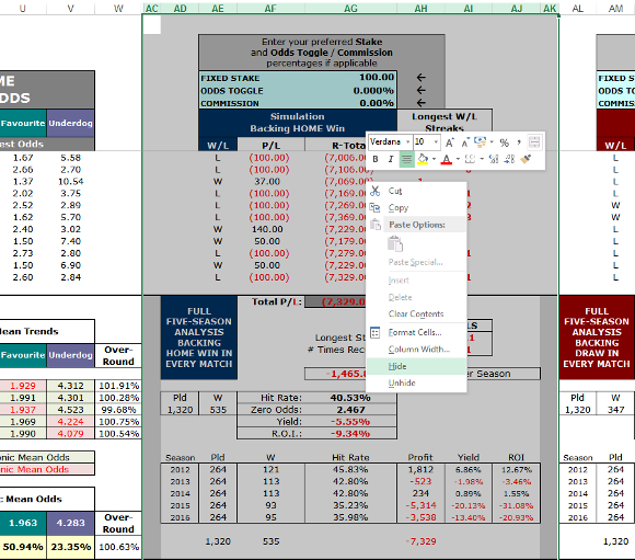
We’re not interested in the home win at the moment so we will hide it, effectively moving the draw data to the left in the spreadsheet.

For the Excel novices amongst you:

• Click on the ‘AC’ label at the top of column V to highlight the whole column.
• Keeping the left mouse button down, draw the cursor across from the letter AC to column AK and then release the button to highlight all of these columns.
• Right click anywhere in the highlighted area and choose ‘hide’.

Here’s a screenshot to ensure you’re on the right track:

If you really want to go minimalistic, you can also hide everything else you don’t need.

The only columns up to column AL that you will need in view are columns P-W inclusive, and the match number in column G.

Sorting

Next, we sort the entire match list by the draw odds in column S.

To select the match list click on the bottom row of data. You will see in this example that the last row of data is numbered 1329. Left click on the number 1329 to highlight the entire bottom row. Here’s a snapshot.

(Click on the images below to enlarge them in a new tab):

Scroll to the top of the list. Hold the shift key down and left click on the number 10 (the tenth row). The whole data field should now be highlighted:

Click on the Data tab at the top of the spreadsheet (between Formulas and Review). Click on Sort. You will be prompted to enter a password, which is 123. (Passwords for all protected areas of the workbook are shown in the Legal Tab).

Click on ‘OK’. A new box will appear:

As we are sorting by the draw odds in column S, make sure this is set in the ‘Sort by’ box and check that under ‘Order’ you are sorting from the smallest to largest value. This will provide us with the definitive list of match data sorted by draw odds in ascending order.

Filtering

We are looking at odds between 3.32 and 3.65.

We now need to hide the portions at either end of this scale. In other words, all matches with draw odds up to and including 3.31, and all those above 3.65.

Do this in the same way as before. Find the row that corresponds with the last value of 3.31. In our example, this is row 106:

Hide rows 10 to 106. Select the rows as we did before and then right click anywhere in the highlighted area. Choose ‘hide’.

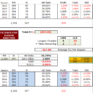
Carry out a check that our first inflection point, 3.32, is in fact in profit. Our example reveals that there were only four games in five seasons with draw odds of 3.32, and only one of these won. This odds cluster is not profitable and we can now hide rows 107-110 as we don’t need them.

Look at the next set of odds, 3.33. Rows 111-116 show six games played with these draw odds. Three won and three lost, but there is healthy profit as a result.

Our first inflection point is therefore adjusted to 3.33.

You may need to look at more than a couple sets of odds in this fashion until you find the first one in profit. These small adjustments are needed because Excel can only handle a maximum of 200 data sets (clusters) when compiling a graph, and match lists rarely divide equally into groups of 200.

Our list here is 1,320 matches long, which would mean 6.6 matches in each split. We therefore need to check exactly where the cut-off points are. The Inflection Point graphs tell us where to look, and the Data Tab sorting and filtering exercise allows us to be more accurate identifying where the inflection points really are.

Our data list now starts on row 111 at odds of 3.33.

We repeat this exercise to find the other end of the scale. We hide everything from the largest odds at the bottom of the spreadsheet up to odds of 3.65:

As you can see, odds of 3.65 do not create a profit over five seasons. Nor do 3.64. The first odds that do are 3.63. We therefore adjust the sorting exercise as before and hide everything up to 3.63.

Our data list now ends on row 666 at odds of 3.63.

Important: The very last thing to do now is select (highlight) the remaining data list and sort it by column G (match number), to put everything back into chronological order. (This time you won’t need a password).

We need to do this to ensure accurate calculations of the winning and losing streaks.

Next Page: Step 3 – Adjusting the Filtered Five Season Analysis Box

About the Author

The Holding Midfielder

Administrator

Not here for flashy wins. Here to read the game. I help bettors see the patterns, protect their bankroll, and play the long game—just like any good holding midfielder.!

View All Posts